Physical Acoustics Lab

Below are short descriptions of research projects available for postgraduate students in our group at the University of Auckland. If you are interested in any of these, please contact us for technical questions. For questions around enrollment at the University of Auckland, please go here. Scholarships may be available for the best applications through the University of Auckland, or the Dodd Walls Centre.

the Auckland volcanic field

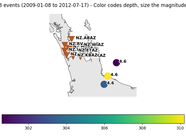
We have a Marsden Fund Grant to study the Auckland Volcanic Field, with funding for a PhD and an MSc student in seismology. There are opportunities for field work on land and at sea.

Background:

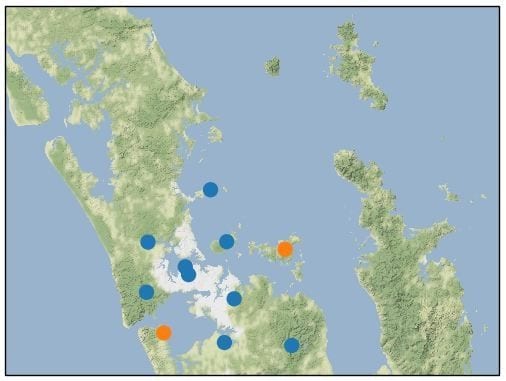
Auckland, New Zealand’s largest city, sits on an active, monogenetic, and intraplate volcanic field. An international team of geoscientists from New Zealand, the USA, and China have joined forces to investigate why this volcanic field exists. An on- and offshore temporary seismic network will provide the density and the aperture of sensors to create the first high-resolution three-dimensional image of the Auckland Volcanic Field (AVF) from the surface to deep in the Earth’s mantle, beyond the depths of the magma that feeds the AVF. The resulting image will then constrain geodynamic modelling of mantle flow to explain what controls the AVF, and with it, this class of intra-plate volcanic fields.

ResonanT Ultrasound Spectroscopy

Resonant ultrasonic spectroscopy fills an important gap between our ultrasonic and seismic research. Together with the PORO lab, we have rock samples to complement laser ultrasound and a host of other petrophysical data with new RUS results.

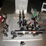
Laser ultrasonic rock physics under high pressure and temperature

The PAL and PORO lab join forces by combining our respective strengths in laser ultrasound and rock physics to improve data quality and quantity. In this project, we are building the expertise to do laser ultrasound in a pressure vessel with optical windows. Source/receiver locations are varied under computer control with an arduino-controlled servo rotational stage.

quality control of timber and fruit products with laser ultrasound

Laser ultrasound can be applied to products of interest to a wide community. Current methods of testing the quality of fruit and timber, for example, can often be described by one or more of the following terms: sparse, contacting, expensive, and often destructive. In this project, we aim to explore the opportunities for laser ultrasound in estimating the quality of  fruit and timber in a non-contacting and non-destructive matter.

Numerical modelling and experiments in photoacoustic (medical) imaging

The stations of the seismic network that monitors the Auckland Volcanic Field are a mix of surface and borehole seismographs. Our aim here is to figure out the orientation of the three orthogonal components of each seismometer.

The vertical component

The vertical components of the seismic network are tested with some earthquakes with an epicentre that is only a ~100 km from the AVF. These are very deep earthquakes, assuring that high-frequency signal impinges from below on the network.

The figure below shows that seismic data from these events generally results in an arrival with a negative maximum, except stations KBAZ and WTAZ:

From this example and seismic data from other earthquakes, we conclude the polarity on the vertical component is reversed for stations KBAZ and WTAZ.

The horizontal components

The majority of the seismic stations in the AVF are in boreholes between 50 to 400 m deep. Particularly for these stations,  the orientation of the horizontal components of the each station is unknown. Luckily, there are several techniques to estimate the orientations of the orthogonal horizontal components.

Ambient Noise Orientation

Stachnik et al. (2012) used a earthquake-sourced Rayleigh wave polarisation method to estimated the orientation of ocean bottom seismometers. Zha et al. (2013) used ambient seismic noise, applying a polarisation technique to the Rayleigh wave signal in CCFs to estimate the orientation of ocean-bottom-seismometers. Here we use ambient noise orientation, based on the method used by Zha et al. (2013), but we use it for borehole seismometers. We performed ambient noise orientation on all 3-component seismometers in the network, using the surface stations as a control group. The  method involves three basic stages:

This method involves three stages:

1.  Computing the three-component cross-correlation functions for all station pairs from noise.
2. Measurement of sensor orientation through an optimization process.
3. Data selection and statistical analysis to obtain final orientation angles.

three-component cross-correlation functions

Cross-correlation functions (CCFs) can be computed for any pairs of seismic sensors. Computing all the possible cross-correlation functions for a pair of three-component seismometers would produce nine functions. For this technique, we use some of the CCFs that potentially contain Rayleigh wave signal. Rayleigh wave motion occurs in the vertical plane so we expect virtual Rayleigh wave signal to emerge in the vertical-vertical(C_zz), and the radial-vertical (C_rz) CCFs. For seismometers with unknown orientation, the C_rz data is distributed across the horizontal-verticals (C_1z and C_2z) cross-correlation functions.

Optimisation

For each pair of seismometers, the symmetric CCFs are bandpass filtered to the frequency band where Rayleigh wave with the greatest amplitude are expected to emerge (In our case 0.05–0.5Hz). We then perform a grid-search through 360-degrees, each performing as an estimate of the angle that would rotate C_1z and C_2z into the C_rz and C_tz . For each estimate of C_rz,  the zero-lag cross-correlation and coherence between the C_rz and 90-degrees phase-shifted C_zz is computed. The maximum cross-correlation marks the best estimate of C_rz. The coherence at maximum cross-correlation is used in the data selection. The back azimuth can then be calculated because the coordinates of both stations are known.

The figure below this process is illustrated for the AWAZ-ABAZ pair. On the left, there is C_zz, C_1z, and C_2z, and the phase shifted C_zz in the dashed red. In the middle panel , the correlation and coherence are plotted by angle. On the right, there is C_zz, and the C_rz, and C_tz based on the angle at maximum correlation (260 degrees in this case), and the phase shifted C_zz in the dashed red.

Data Selection and Statistical Analysis

Estimates with a coherence below 0.5 at maximum correlation tend to be scattered to a greater degree. These coherences were discarded. We then take the mean of the remaining estimates as our final estimate of the orientation. In the figure below, the estimates for the AWAZ station are presented in a polar plot. The radial axis represents the number of estimates in each 1-degree bin. Red represents estimates with coherences below 0.5 that are removed.

Stachnik, J.C., Sheehan, A.F., Zietlow, D.W., Yang, Z., Collins, J., & Ferris, A., 2012. Determination of New Zealand ocean bottom seismometer orientation via Rayleigh-wave polarization. Seismological Research Letters, 83(4).

Zha Y, Webb SC, & Menke W. Determining the orientations of ocean bottom seismometers using ambient noise correlation. Geophysical Research Letters. 2013 Jul 28;40(14).

The key idea behind ambient noise seismology is to focus purely on the seismic noise that was once removed in traditional seismology. Incoming signals from 11 seismic stations across Auckland are filtered to look at frequencies attributed to ocean noise. This noise is continuous so measurements can be taken constantly.  The Auckland volcanic field (AVF) is ideal to study with this technique as we have oceans on both sides, creating a relatively even distribution of noise in the earth beneath us, hence we say that the AVF has a pseudo isentropic wavefield.  

11 stations comprising the Auckland seismic station network

 Waveforms from two stations are filtered at the frequencies associated with ocean noise and sliced into smaller chunks known as stacks. One waveform is moved relative to the other and the similarity or correlation is measured between them. A plot of the similarity against the time shift creates a Green’s function. This is done for each of our chunks and is added together to create an impulse response between the two stations for each day.  

Green’s function between Awhitu and Waiheke Island

Above is an example of a Green’s function between the Awhitu station and the Waiheke Island station (shown as orange dots on the map above). The right side (positive lag time) shows the impulse response as if there was a quake at the Awhitu station as seen from the Waiheke station and the left hand side shows the response at the Awhitu station as if there was a quake at the Waiheke station. Notice the virtual quake coming from the Awhitu side is larger than that from the Waiheke station. This is because the Awhitu station is closer to the West Coast, which is a strong source of ambient ocean noise, so it’s virtual earthquake appears larger. Dispersion can also be observed with low frequency waves arriving first. These waves have a greater wavelength, so travel through deeper parts of the earth where they can travel faster. MSNoise.org provides a suite of tools in Python to calculate the wave fields of these “virtual earthquakes” between each combination of station pairs of the Auckland network. 

 The time it takes for this impulse to go from station to station can be determined by looking at the Green’s Function. In this example it takes about 25 seconds for surface seismic waves to travel from Awhitu to Waiheke and vice versa.  

To use this method as a monitoring tool a reference is created to show what a normal Green’s function looks like. Then our data for a set period of time is stacked. A short stack ( ie 1 or 2 days) will have more small fluctuations whereas larger stacks shows larger trends more clearly but lack the resolution to see short term impacts. These stacks are compared to the reference. Below is a plot of the change in seismic velocity over the last 6 months for different stack lengths. Shorter stack lengths appear to have more random fluctuations whereas the 30 day-long stack at the bottom allows smoother trend to be seen. A decrease in seismic velocity in October and an increase going into December can be observed. 

Seismic velocity variation for the Auckland Volcanic Field between August 2018 and January 2019

Link to up-to-date dvv plots for the AVF.

There are a number of possible explanations for changes to surface seismic velocities.  For example, on Mount Merapi, Indonesia, changes in the waveforms correlate with changes in precipitation saturating the near-surface. However, in principle magmatic changes could be detected this way. Areas of active research include how to do the calculations so that we can exclude causes for changes in the waveforms not related to the Earth. For example, the distribution of noise sources may vary from day to day, affecting the calculated “virtual earthquakes.” 

This blog will describe the running of FMTT on the AVF.

INSTALLATION

The installation was done by following the instructions obtained from

http://rses.anu.edu.au/~nick/teletomo.html

In fact, all the necessary files are attainable in an all in one download as a compressed Unix gzipped and tarred file specified in that link. In which it includes the instruction manual, a research paper of its application, and a couple of examples.

In a nutshell, to install all we need to do is to run the shell script compileall after the compressed file has been unpacked. But for things to run smoothly, prior to running the shell script what we did was:

• Edit line 22 of  compileall and line 5 of source/aktimes/Makefile into the appropriate Fortran compiler. In my case this is gfortran.
• Still in compileall, add ./ before remodl and setbrn in line 82 and 83 respectively so that these can be found during compilation.
• Edit line and line 19 and line 181 of syntht.f90 source file. Delete (KIND=i10) in both lines to avoid mismatch of function error.

Compilation complete

FMTT itself consist of several individual executable programs. Each one requires an input file which name is identical to the executable except for the .in extension. In these input files we can specify and modify the parameters so that the desirable inversion routine is performed. More details on each program can be found inside the instruction manual.

An executable worth to note is tomo3dt, which perform the whole tomographic inversion as opposed to run the necessary executable programs one after the other. Another notable mention is gmtslicet. This program is used to help plot and visualize the inversion result as depth, E-W, and N-S slices. The complete plotting procedure is based on GMT scripts (GMT stands for Generic Mapping Tools).

Running the Example

Two examples were provided in the compressed file. Prior to do any of the examples, ak135.hed and ak135.tbl need to be copied into the respective example directory. These files can be found in source/aktimes after compilation. Once the files are copied, simply execute tomo3dt from the directory. It should returns the following lines:

gugi@sc-9020-hs:~/AVF/fmtt_v1.0/example1$ tomo3dt
Program fm3dt has finished successfully!
Program fm3dt has finished successfully!
Program fm3dt has finished successfully!
Program fm3dt has finished successfully!
Program fm3dt has finished successfully!
Program fm3dt has finished successfully!
Program fm3dt has finished successfully!
Program fm3dt has finished successfully!
Program fm3dt has finished successfully!
Program fm3dt has finished successfully!
Program fm3dt has finished successfully!

The number of times the line “Program fm3dt has finished successfully!” is repeated depends on the number of iteration specified in the tomo3dt.in, the input file for tomo3dt. This shows that we have managed to perform a successful tomographic inversion.

Plotting the Examples

After tomo3dt has been successfully run and the rounding issue in gridi.vtx and gridc.vtx has been adjusted, the results are visualized using gmtslicet and GMT. Go to the subdirectory /gmtplot and execute gmtslicet. Prior to executing gmtslicet, the files gridi.vtx and gridc.vtx might need to be adjusted. In the top lines of both files, the numbers round off differently to each other which could result in an error while running gmtslicet. Equalizing these values will solve the error. Nick Rawlinson kindly provides us with an updated gmtslicet.f90 source file. It meant to tackle the rounding problem. It works in some computer but somehow it could be machine specific.

The execution of gmtslicet will produce three bound .gmt files (among others) for depth, E-W, and N-S strike. These are used by the plotting scripts plotd, plotew, and plotns. Prior to running these scripts, some modification were made. #!/bin/csh was added on the top of each script file. Then, depending on how GMT is called in your computer, gmt may need to be added before each GMT command namely gmtset, xyz2grd, grdimage, psscale, psxy, pscoast. Output file can also be modified.

The results of running the plotting scripts are of .ps file type which can be viewed. Depth or E-W or N-S slice is depicted by their respective script file.