Over the summer and semester 1 of 2019 I have been using MSNoise to monitor the Auckland volcanic field along with several small associated investigations that followed. This page aims to provide a summary of methods, results, possible lines of enquiry for future work as well as questions that are still unanswered after this time.
For my research over summer, a summary can be found here, along with my final report here.
Over this time I created a guide for myself called MSNoise-how-to. It is very informal but is a good place to start for anyone new to MSNoise, filling in some of the spaces left in the documentation and other useful tips I discovered relating to using linux for the first time. A link to this document can be found here.
DVV monitoring tool:
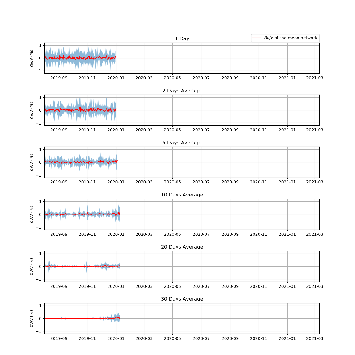
A link to the final output on the PAL website can be found here. A bash script was created to download seismic data, process it using MSNoise to create the dv/v plot and then remove the data once completed. This script was added to the cron file by Guy, and with some SQL help from Josiah, this runs every day to build up a picture of temporal variations of surface seismic waves in the AVF.
The plot updates here everyday: https://nzseis-stations.auckland.ac.nz/pal/
I adjusted the python script from the MSNoise defauly, to add error bars and to make the y-axis of each of the moving-windows the same in an attempt to avoid misleading people who might interpret the result to be a warning sign of a big eruption event . My adjusted version of the code can be found here.
There are still some issues with this tool. The dv/v output has an option to plot the line of best fit’s gradient forced through the origin or not. Ideally the gradient should go through the origin as we would expect a lag time of zero to be associated with zero change from the reference. The key issue here is that that the two plots (M0 (origin forced gradient) vs M (best fit gradient)) are quite different. In an ideal world these should be the same, which indicates issues with the line fitting, possibly that the line is being fitted around points in the wrong region, or our green’s functions for the station pairs are non-sense. By setting the window encompassing the points being fitted to “dynamic”, MSNoise chooses an appropriate window based on station separation, avoiding human errors and adjusting it according to each pair. I suspect that not all station pairs are created equal, with the interstation path being being equidistance from our ambient seismic noise source (the two harbours and coasts of Auckland) and when these stations are averaged to plot the dv/v for the AVF they reduce the quality of the data.
An avenue of investigation would be to determine which station pairs have reliable dt/t plots, giving believable gradients, which are similar to M0, then only using these stations when plotting the data. Another option would be to determine an exemplary station pair, one which has clear greens functions plots, providing accurate dt/t and then dv/v measurements that we can then assume apply to the AVF.

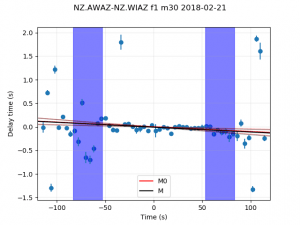
Above is an example of the dt/t plot for a random station pair’s 30 day average (Awhitu to Waiheke Island). The lines of best fit has a very small gradient which is what we want, considering the AVF has not had any reasons to expect elevated dt/t levels. The blue section is the window containing the points that the linear regression is best fitted to. As you can see the delay time gets greater as the lag time increases, so window selection is important to ensure the line of best fit is being created using appropriate points. Just by eye-balling this plot, perhaps the window would be better if moved closer to time=0 to encompass the linear section from time=20 to 50. In this instance perhaps the dynamic window fit is not the best. As this data is a 30 day average, we would expect more uniform points. This large variability in points could also indicate this station pair is not good for making inferences about dv/v in the AVF.
Another avenue of investigation would be to determine what window size and position gives the best line of best fit for a given station pair. Ideally this would have similar results for both M and M0, with a relatively small errors.
dv/v correlations with groundwater level.
This investigation looked to determine if there was a correlation between groundwater levels and temporal seismic velocity in the Auckland region.
Ambient Seismic noise method for dv/v data.
- Data downloaded from Geonet FSDN for the years 2017-2018. This uses all 11 stations in the AVF Filtered at 0.03Hz to 1.0Hz.
- Cross correlations for each day was obtained by sampling every 20s from 10 minute windows, which were then averaged for a daily CC
- These are compared to a reference to obtain the dt/t and then dv/v for each station pair over the two years.
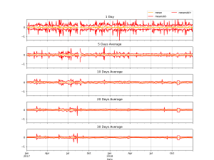
- The dv/v plots are shown using the mean and median of from all station pairs at a number of different window lengths. A value for a given day with a window length x corresponds to the average for x days before the current.
- Before comparison, the dv/v days are shifted by half of their window length so that the day in question is now in the center of the window.
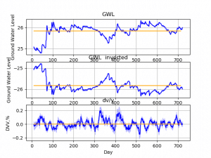
Below is an example of the dv/v plot for all the stations, in the AVF from January 2017 to December 2018.

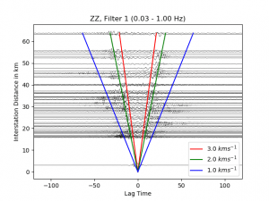
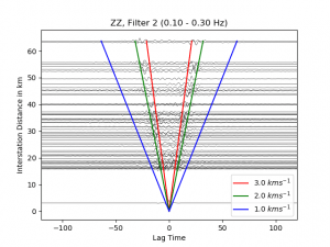
The outputs are highly variable depending on window length, station pairs used, ground water levels sites used and whether M or M0 is used to determine dt/t. Another option depends on the frequency the initial data is filtered at. Below is an example of two different filters in the influence they have on the Green’s function plotted against inter station distance. This difference in green’s function based on different filters will also change the resulting dv/v and then the relationship between the dv/v plot with ground water level data. From the plots below, velocity is best represented by filter 2.

 .
.
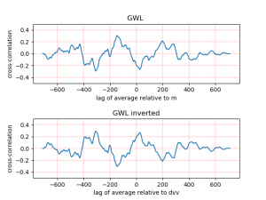
I wrote a script to visually show the correlation between the chosen groundwater level and chosen dv/v data. It can be found here. Below is an example of the output I get from correlating the 20 day average for the NZ_EPAZ_NZ_HBAZ station pair , based on the line of best fit that wasn’t forced through the origin against the average ground water (averaged over 8 ground water level station across the Auckland region).


This plot above is as expected, where there is a positive correlation between change in seismic velocity and the inverted groundwater level. This is because the signals we interpret are predominantly shear waves, whose speed is described by,
V=√(G/ρ); G is shear modulus and ρ is the density of the material.
Rainfall and groundwater increases the density of the earth, so the waves travel slower. There is also a peak at approximately –360 days which shows this is an annual trend, corresponding to the rainier winter months.
Future investigations would look into changing the parameters that influence the dv/v plot in order to maximise the relationship with ground water levels. Ideally the max correlation will be at zero days lag. This would involve getting the best possible representation of dv/v by selecting station pairs that do show groundwater level correlations (ie ones that are not separated by water) etc. Also I would further investigate which specific ground water sites reflect the seasonal variation and use these to create a better, more accurate representation of seasonal groundwater.
The result of this experiment varied wildly depending on the station pair, filter, window length and choice of gradient in dt/t plts (M vs M0), so there is a lot of work that could be done to determine which parameters offer the most accurate method of obtaining a dv/v plot that reflect changes in ground water level. Also we could prove this method by showing there is no correlation between groundwater level and dv/v plots with paths that pass primarily through the ocean.
