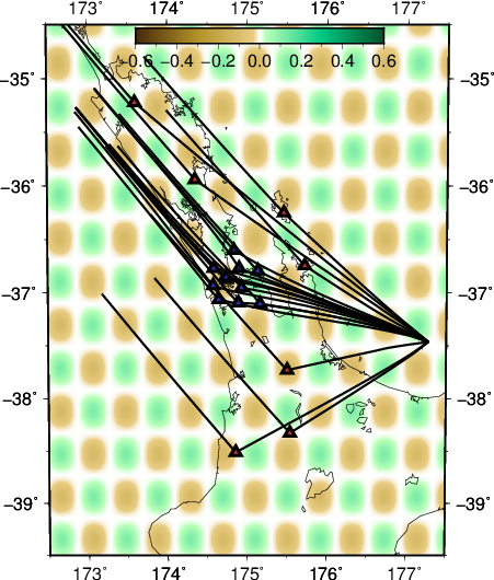
Our results in regards to the checker-board tests show convincing observations. However there are still work to be done in terms of the data fitting. The joint inversion misfits do not reflect the good misfit of local and teleseismic event inversion individually.
One sample
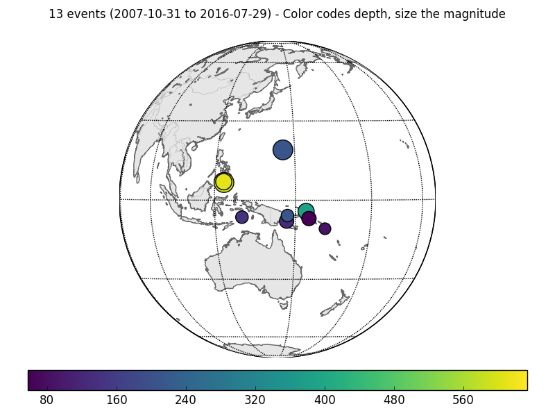
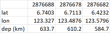
In order to see the behaviour of the joint inversion, we start with the simplest case of jointly invert one local and one teleseismic event.
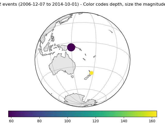
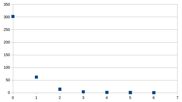
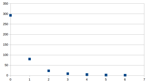
Individually inverting each event shows that the misfit can be minimized. For a single source this is theoretically expected. For the local source inversion, after six iterations, the rms misfit reaches 0.46 ms. Whereas for teleseismic source, after six iterations, the rms misfit reaches 1.84 ms.
-
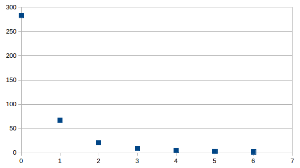
- RMS residual in milisecond versus iteration for local (top) and teleseismic (bottom) inversion using one sample each
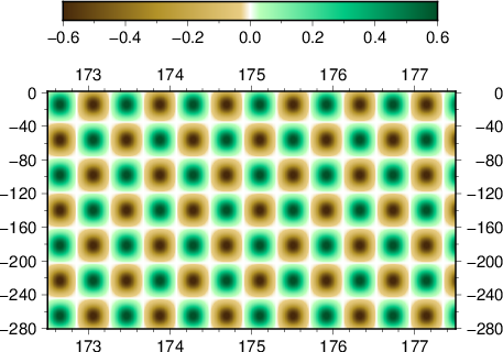
The corresponding models are as follow:
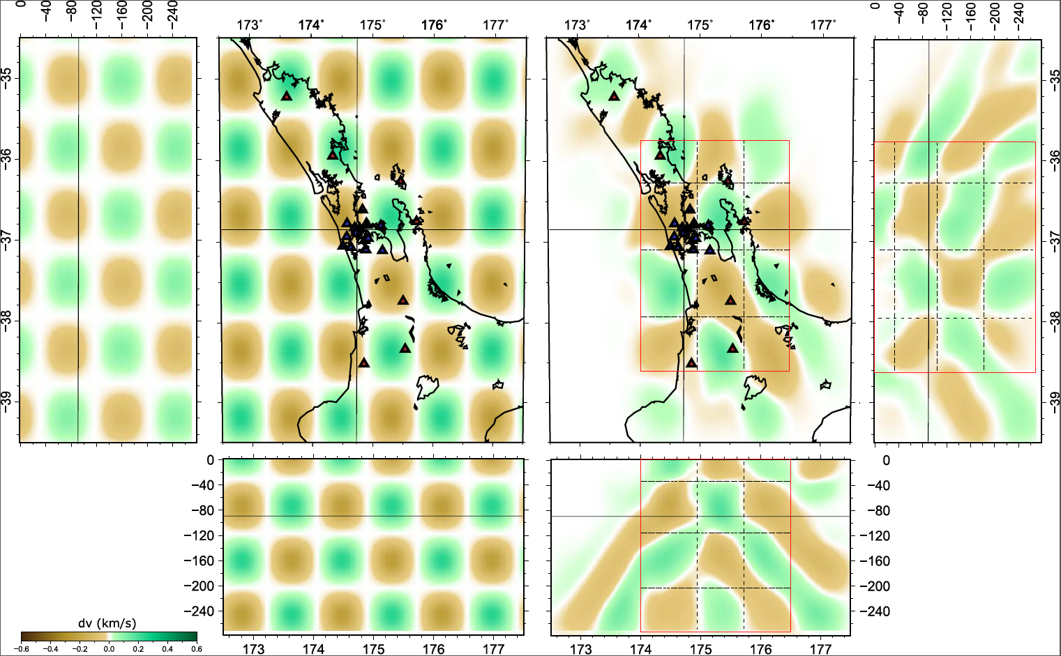
-
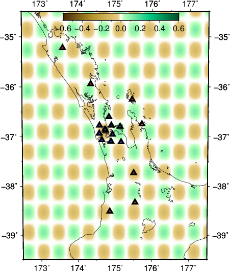
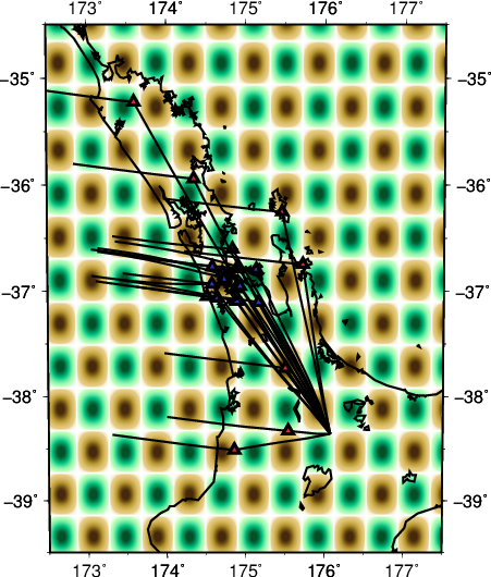
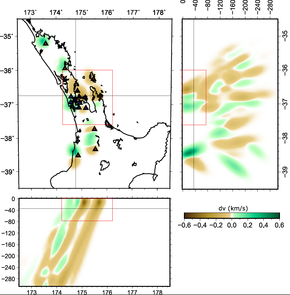
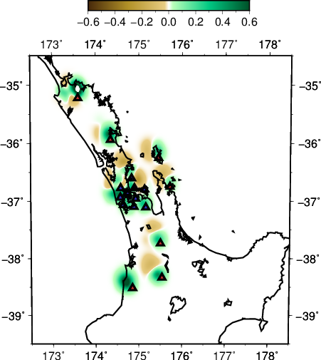
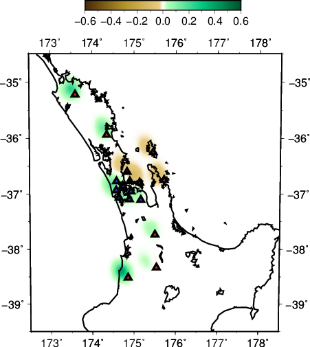
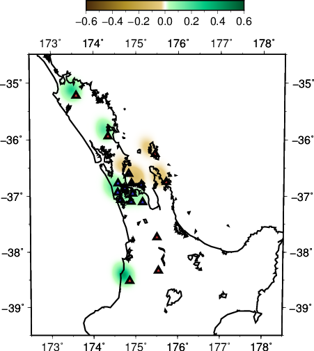
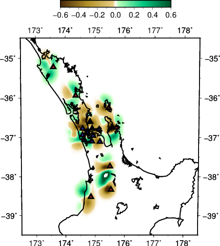
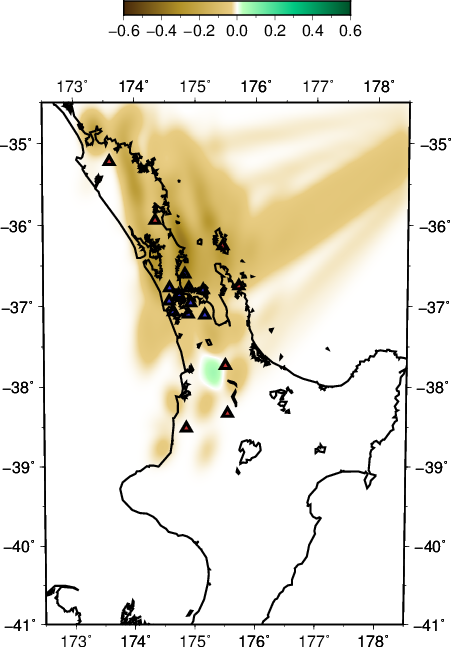
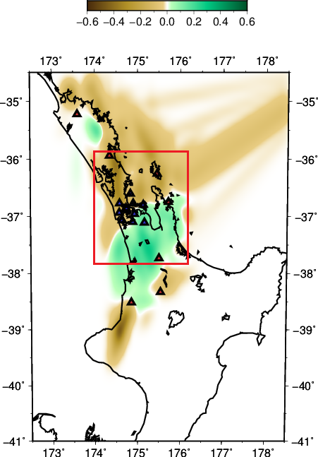
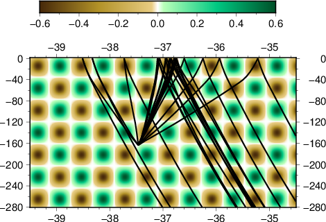
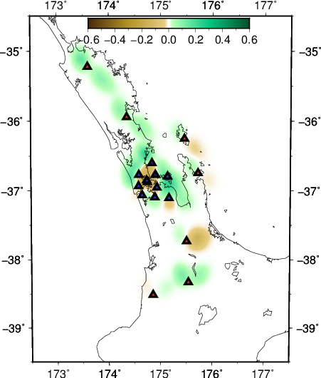
- depth slice at 30 km
-
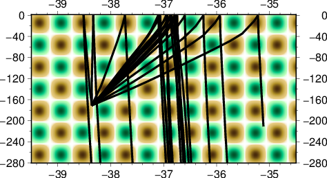
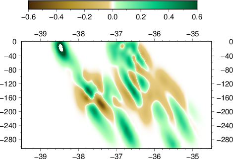
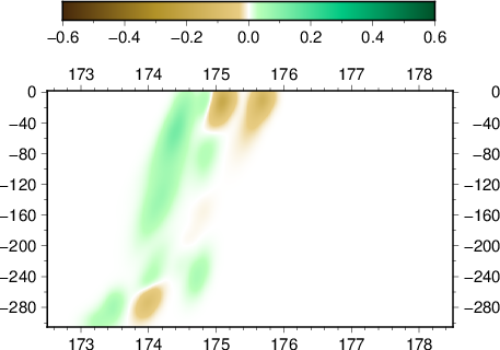
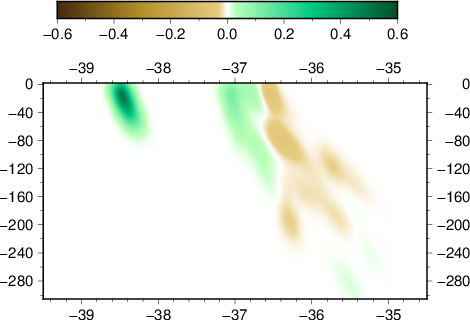
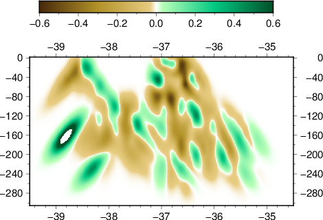
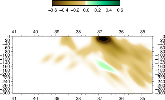
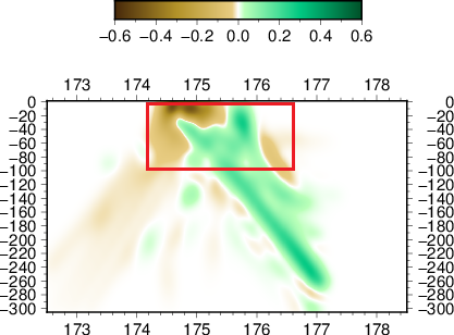
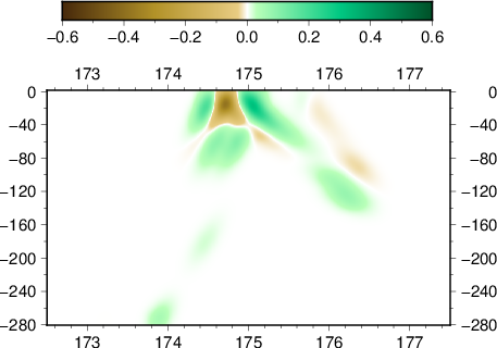
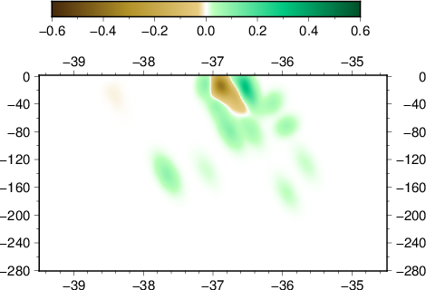
- EW slice at 36.85 S
-

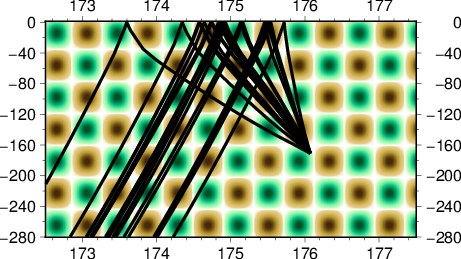
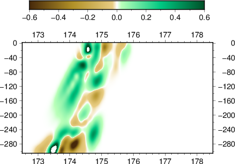
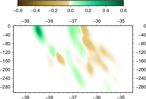
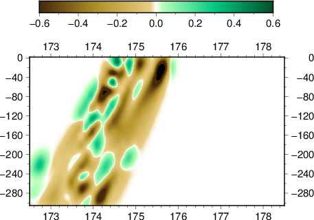
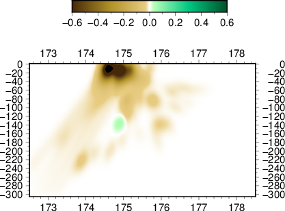
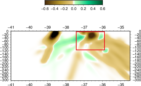
- NS slice at 174.75 E
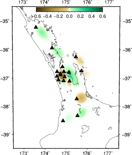
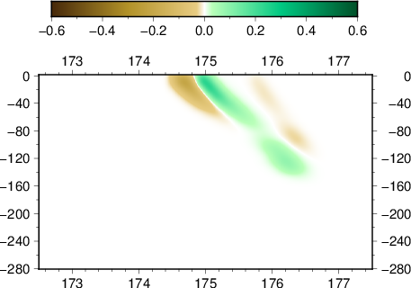
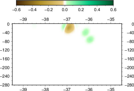
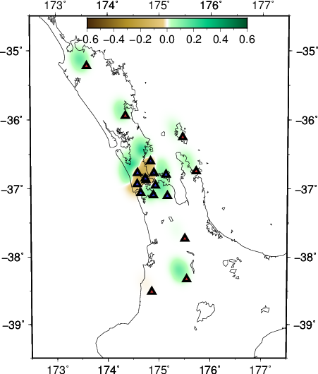
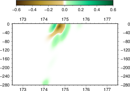
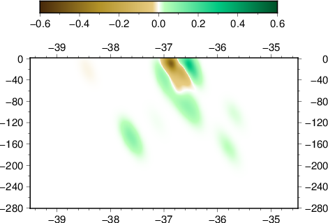
Where the first three are the initial model, the middle three are for the local event inversion, and the bottom three are for the teleseismic event inversion.
Next is to see the trend in misfit when the two events are inverted jointly. Since the events are coming from different directions, there should not be any conflicting information with regards to raypaths, so we expect the misfit to be similarly small.

Results shows that this is indeed the case, where the rms misfit after six iterations reaches 1.37 ms. This observation does not indicate a deterioration in data fit while performing a joint inversion of a single local and teleseismic source.
joint inversion – rms residual (millisecond) vs iteration
The recovered model is also improved accordingly.
-
- depth slice at 30 km
-
- EW slice at 36.85 S
-
- NS slice at 174.75 E
Adding events
Adding one more local source to be inverted does not reduce the misfit significantly. After six iterations, rms misfit reaches 1.52 ms. On the other hand, adding another teleseismic event on top of that doubles the misfit to 3.22 ms, albeit this value is still very small.

4 events inverted
We keep adding more events. Additional local source (5 in total) produce a misfit of 3.02 ms, slightly less than 4 sources inversion. If on top of that we invert an extra teleseismic source (6 in total), the rms value goes to 4.25 ms. So far, it seems that the highest influence in terms of increasing the misfit has been in relation to the addition of teleseismic source.
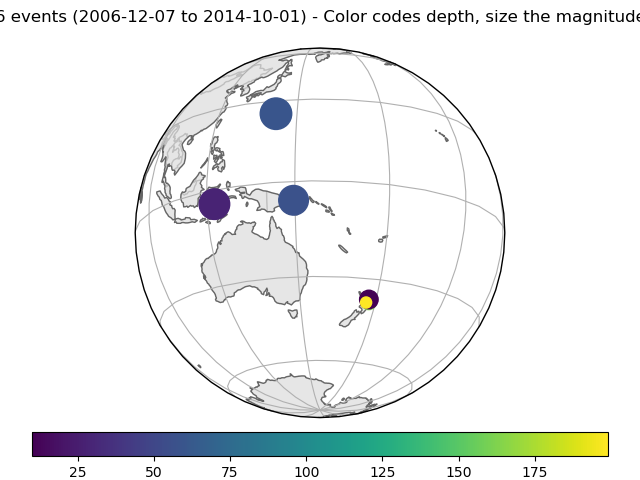
6 events
Misfit trend
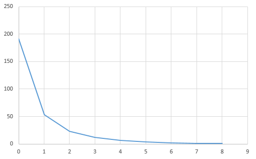
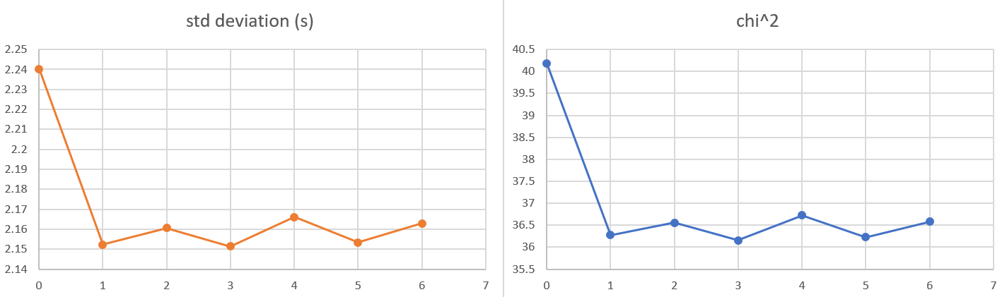
We would like to show the progression of the misfit of the data with the addition of events for local sources only. We show here the rms residual in millisecond after six iterations using varying number of local sources starting from 1 event increasing to 2, 5, 10, 50, and 100 events. Consistently in all cases we turn the regularization off by making eta and epsilon equal to zero.

(table) 6 iterations rms values for varying number of sources
| 1 | 2 | 5 | 10 | 50 | 100 | |
| 0 | 302.25 | 232.17 | 245.38 | 231.66 | 250.63 | 261.3 |
| 1 | 61.99 | 42.75 | 45.35 | 58.04 | 64.75 | 75.62 |
| 2 | 13.85 | 10.25 | 12.42 | 18.14 | 25.81 | 32.31 |
| 3 | 3.76 | 3.38 | 5.5 | 8.79 | 14.77 | 19.17 |
| 4 | 1.49 | 1.8 | 3.28 | 5.96 | 10.98 | 13.91 |
| 5 | 0.8 | 0.77 | 2.25 | 4.39 | 9.61 | 11.42 |
| 6 | 0.46 | 0.61 | 1.58 | 3.29 | 8.46 | 9.78 |
Visually, we see that apart from the one source inversion, from 2 sources to 100 sources the lines corresponded to the rms residual improvement are shifted upward with the addition of more sources. This seems to imply that progressively the misfit shy away from zero with the inclusion of extra sources in the inversion.