In this travel-time tomographic inversion we plan to use more events to get a significant result in terms of AVF subsurface velocity field.

stations

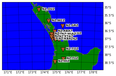
Eighteen stations are used in the inversion. These are divided into 11 stations located around the central area, and 7 outer surrounding stations. We removed the low resolution channels associated with the station.

events and picks

We have 116 earthquakes around the region that we plan on using.

Almost all events have good trace data, which means that we have a good quality source input that we can work with. Our next step is to determine the first arrival pick with impeccable accuracy. The automatic trigger does a good job with picking the arrivals to a couple of seconds or so, but to consistently get an accuracy to the second or even less, picking by hand is still the go to method.

While we are doing the picking, some number of traces don’t show the event. We presume that this is mostly due to the location of the related station. The relative distances can make the time window in which the traces are shown becoming too short. For example, the northernmost station OUZ is the one that mostly show this condition. For the following results, the corresponding picks are excluded from the inversion, but we can revisit these picks and include them later on.

Even though the number of traces that don’t show an earthquake is small, it is still small things that we can improve on.

inversion

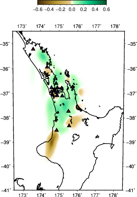
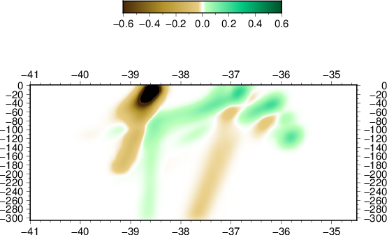
The split in the positive and negative anomaly (in km/s) which we also saw in the inversion with less events can be seen more distinctly this time around. Positive anomaly is prominent to the North and similarly, negative in the South. Another highlight is the negative anomaly right below Auckland (36.6-37.2 S, 174.6-175.2 E) at 50+ km.

We can even see a dip in the anomaly although we cannot be sure how much influence does the smearing effect has here. It is consistent with the primary paths direction from the South-East. However unlike any smearing that we have seen before in previous results, that are usually constricted to the outer and deep part of the model, here it is rather central. For example, the deep lineaments in the NS slice are likely to be smearing, and are in agreement with the three deepest events. Furthermore, our previous analysis from the checker-board test shows that at least for the first 70 km or so, the smearing is not too dominant. Therefore, we may be seeing a jump or a continuation of structure to depth commencing somewhere in the south Auckland.

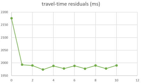
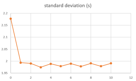
Here are the plots showing how the root-mean-square travel-time residuals, standard deviation, and chi^2 change through each iteration. The first iteration is when the misfit drops drastically, afterward the plots quickly becoming stable. These plots justify the number of iterations we did as after three or four iterations we already have a convergence.

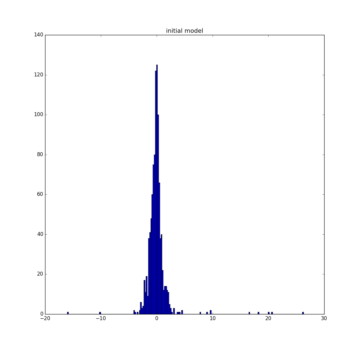
We have here the histogram of the travel-time residuals for initial and final model. There is no change between the two, but that is consistent with the standard-deviation plot. Most residuals are within a couple of seconds, but we do have some that can be more than 20 s late.