The key idea behind ambient noise seismology is to focus purely on the seismic noise that was once removed in traditional seismology. Incoming signals from 11 seismic stations across Auckland are filtered to look at frequencies attributed to ocean noise. This noise is continuous so measurements can be taken constantly.  The Auckland volcanic field (AVF) is ideal to study with this technique as we have oceans on both sides, creating a relatively even distribution of noise in the earth beneath us, hence we say that the AVF has a pseudo isentropic wavefield.  

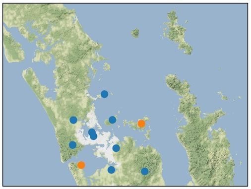
11 stations comprising the Auckland seismic station network

 Waveforms from two stations are filtered at the frequencies associated with ocean noise and sliced into smaller chunks known as stacks. One waveform is moved relative to the other and the similarity or correlation is measured between them. A plot of the similarity against the time shift creates a Green’s function. This is done for each of our chunks and is added together to create an impulse response between the two stations for each day.  

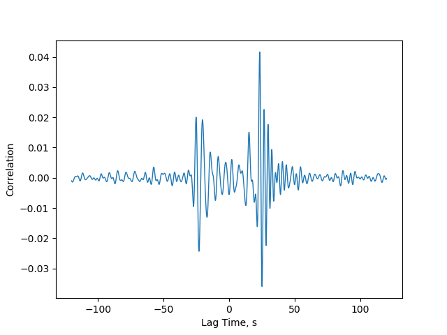
Green’s function between Awhitu and Waiheke Island

Above is an example of a Green’s function between the Awhitu station and the Waiheke Island station (shown as orange dots on the map above). The right side (positive lag time) shows the impulse response as if there was a quake at the Awhitu station as seen from the Waiheke station and the left hand side shows the response at the Awhitu station as if there was a quake at the Waiheke station. Notice the virtual quake coming from the Awhitu side is larger than that from the Waiheke station. This is because the Awhitu station is closer to the West Coast, which is a strong source of ambient ocean noise, so it’s virtual earthquake appears larger. Dispersion can also be observed with low frequency waves arriving first. These waves have a greater wavelength, so travel through deeper parts of the earth where they can travel faster. MSNoise.org provides a suite of tools in Python to calculate the wave fields of these “virtual earthquakes” between each combination of station pairs of the Auckland network. 

 The time it takes for this impulse to go from station to station can be determined by looking at the Green’s Function. In this example it takes about 25 seconds for surface seismic waves to travel from Awhitu to Waiheke and vice versa.  

To use this method as a monitoring tool a reference is created to show what a normal Green’s function looks like. Then our data for a set period of time is stacked. A short stack ( ie 1 or 2 days) will have more small fluctuations whereas larger stacks shows larger trends more clearly but lack the resolution to see short term impacts. These stacks are compared to the reference. Below is a plot of the change in seismic velocity over the last 6 months for different stack lengths. Shorter stack lengths appear to have more random fluctuations whereas the 30 day-long stack at the bottom allows smoother trend to be seen. A decrease in seismic velocity in October and an increase going into December can be observed. 

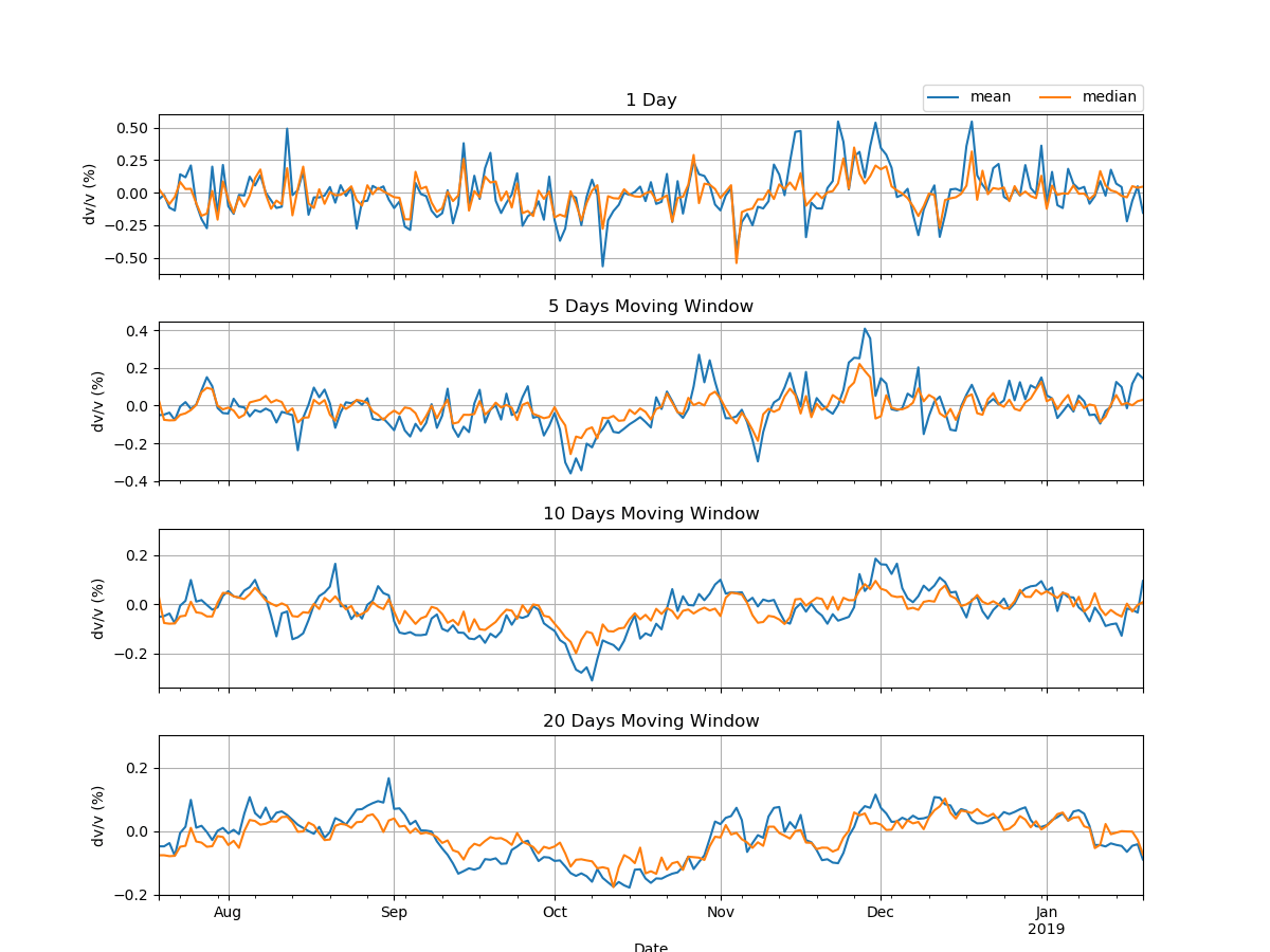
Seismic velocity variation for the Auckland Volcanic Field between August 2018 and January 2019

Link to up-to-date dvv plots for the AVF.

There are a number of possible explanations for changes to surface seismic velocities.  For example, on Mount Merapi, Indonesia, changes in the waveforms correlate with changes in precipitation saturating the near-surface. However, in principle magmatic changes could be detected this way. Areas of active research include how to do the calculations so that we can exclude causes for changes in the waveforms not related to the Earth. For example, the distribution of noise sources may vary from day to day, affecting the calculated “virtual earthquakes.”