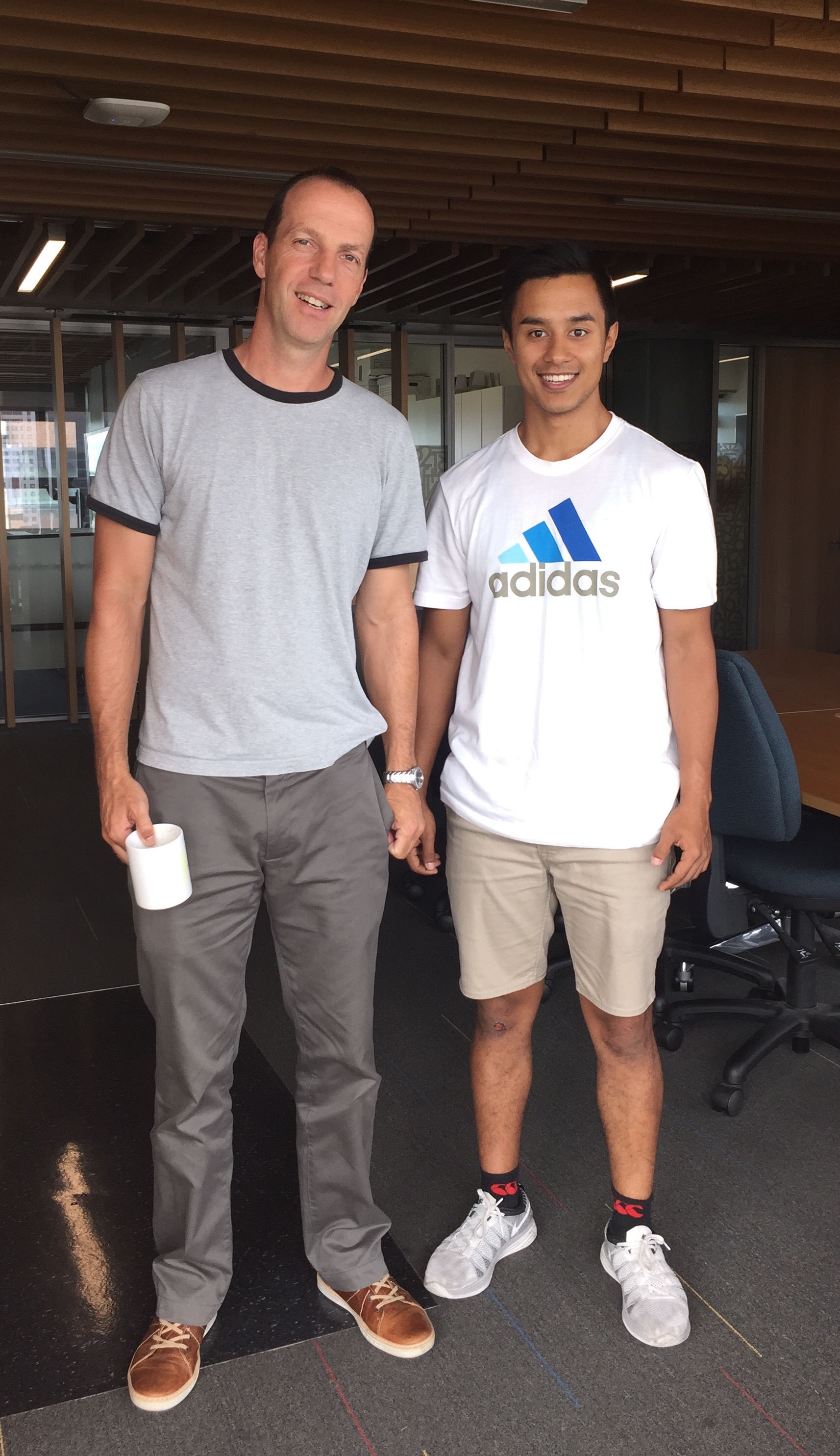
Prabhat Shrestha has embarked on a new adventure with the Schlumberger Gould Research, in Cambridge (UK), after handing in his MSc thesis on microseismic event relocation. It has been a great privilege to have Prabhat in our group. We are proud of all he has accomplished and wish him all the best in England!
Category: PALNews (page 7 of 9)
This (kiwi) Summer, we were lucky enough to have Evan Rust from Boise join the PALs. Evan designed and developed a scanning system for our lasers, and implemented this into our data acquisition system, based on the PLACE open-source acquisition software suite. This ends a year-long work/holiday programme for Evan, and we wish him safe travels on his way back to the US!
After completing his BSc Honours degree with us on time-lapse measurements of carbonate-cemented sandstones, Jackson is starting PhD in the Geophysics Department of Stanford University. We want to congratulate another one of our students heading off to Stanford, where he will join former PALs Leighton Watson and Randi Walters.
A paper by Jami L Johnson, Kasper van Wijk, and Henrik tom Wörden was recently published in the Journal of Laboratory Automation describing the Python package we’re developing. The package is open-source, freely available, and designed for all things experimental: instrument automation, data acquisition, and data analysis. Check out the paper or contribute to the project!
Dr Ludmila Adam (Mila) was awarded one of the very prestigious 2014 Marsden grants from the Royal Society of New Zealand for her proposed research on rock physics of the Alpine Fault. The title of her work is “Getting inside the earthquake machine: fine-scale imaging of the Alpine Fault zone,” and her collaborators are Dan Faulkner, Virginia Toy and John Townend. Congratulations to this team!
In January 2015, The third edition of “A guided Tour of Mathematical Methods for the Physical Sciences” will be available in stores! This book, written by Roel Snieder and Kasper van Wijk, aims to teach mathematical physics by doing lots of fun exercises on a variety of applications in (geo)physics. Roel and Kasper thank all our friends, family and colleagues who contributed in one form or another. Many of them are PALs.
To avoid grainy graphics and the wrong size/type of fonts in publications and presentations, inkscape has a wonderful option, created by Johan Engelen, that splits a figure into the drawing alone and a small latex file that calls the drawing and places all fonts. When you now embed the latex file in your presentation or your publication, the latex style file will determine the size and type of the font used. The result is a perfectly embedded figure in the style of your document! Below are the steps to Nerd Nirvana:
Draw your figure
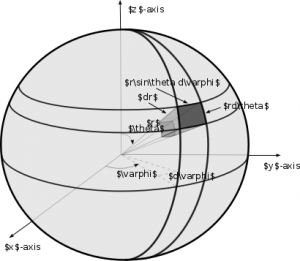
Let’s draw a figure. Here is a figure in svg-format, made in inkscape:
Note that we use latex math commands here, which makes this figure looks a bit messy, at first. When we are done drawing, we save as a pdf, and choose the option: “pdf+latex.” The font-free pdf file is spherefigc2.pdf, and the latex file that places the fonts in it, is
%% Creator: Inkscape inkscape 0.48.5, www.inkscape.org
%% PDF/EPS/PS + LaTeX output extension by Johan Engelen, 2010
%% Accompanies image file 'spherefig2c.pdf' (pdf, eps, ps)
%%
%% To include the image in your LaTeX document, write
%%   input{<filename>.pdf_tex}
%%  instead of
%%   includegraphics{<filename>.pdf}
%% To scale the image, write
%%   defsvgwidth{<desired width>}
%%   input{<filename>.pdf_tex}
%%  instead of
%%   includegraphics[width=<desired width>]{<filename>.pdf}
%%
%% Images with a different path to the parent latex file can
%% be accessed with the `import' package (which may need to be
%% installed) using
%%   usepackage{import}
%% in the preamble, and then including the image with
%%   import{<path to file>}{<filename>.pdf_tex}
%% Alternatively, one can specify
%%   graphicspath{{<path to file>/}}
%%
%% For more information, please see info/svg-inkscape on CTAN:
%%   http://tug.ctan.org/tex-archive/info/svg-inkscape
%%
begingroup%
  makeatletter%
  providecommandcolor[2][]{%
    errmessage{(Inkscape) Color is used for the text in Inkscape, but the package 'color.sty' is not loaded}%
    renewcommandcolor[2][]{}%
  }%
  providecommandtransparent[1]{%
    errmessage{(Inkscape) Transparency is used (non-zero) for the text in Inkscape, but the package 'transparent.sty' is not loaded}%
    renewcommandtransparent[1]{}%
  }%
  providecommandrotatebox[2]{#2}%
  ifxsvgwidthundefined%
    setlength{unitlength}{565.85061095bp}%
    ifxsvgscaleundefined%
      relax%
    else%
      setlength{unitlength}{unitlength * real{svgscale}}%
    fi%
  else%
    setlength{unitlength}{svgwidth}%
  fi%
  globalletsvgwidthundefined%
  globalletsvgscaleundefined%
  makeatother%
  begin{picture}(1,0.5817873)%
    put(0,0){includegraphics[width=unitlength]{spherefig2c.pdf}}%
    put(0.34077896,0.28258916){color[rgb]{0,0,0}makebox(0,0)[lb]{smash{$r$}}}%
    put(0.58016112,0.22314528){color[rgb]{0,0,0}makebox(0,0)[lb]{smash{$y$}}}%
    put(0.02588695,0.05284654){color[rgb]{0,0,0}makebox(0,0)[lb]{smash{$x$}}}%
    put(0.26925349,0.33843429){color[rgb]{0,0,0}makebox(0,0)[lb]{smash{$theta$}}}%
    put(0.20743185,0.09461795){color[rgb]{0,0,0}makebox(0,0)[lb]{smash{$varphi$}}}%
    put(0.51123087,0.43150768){color[rgb]{0,0,0}makebox(0,0)[lb]{smash{$ {bf hat{boldsymbolvarphi}}$}}}%
    put(0.45832621,0.49970874){color[rgb]{0,0,0}makebox(0,0)[lb]{smash{${bf hat{r}}$}}}%
    put(0.47736687,0.29366584){color[rgb]{0,0,0}makebox(0,0)[lb]{smash{$ {bf hat{boldsymboltheta}}$}}}%
    put(0.18005551,0.55995116){color[rgb]{0,0,0}makebox(0,0)[lb]{smash{$z$}}}%
    put(0.25781455,0.40019168){color[rgb]{0,0,0}makebox(0,0)[lb]{smash{$(x,y,z)$}}}%
  end{picture}%
endgroup%
All that is left to do, is import this into your main latex file:
begin{figure}
    import{newfigs/}{spherefigc2.pdf_tex}
  caption{Definition of the geometric variables for an infinitesimal
    volume element $dV$ in spherical coordinates.}
  label{Sphere.figc}
end{figure}
where the end result, looks like this:
this is a low-grade snapshot of a page of our book, but if you want to see the vectorised plot, click here.
Exporting the complete figure
Some editors of journals or books may not be set up to do this dynamic handling of fonts in figures. For them, you can “export” to a pdf file with the (correct) fonts statically embedded, you can use the package standalone.cls. Note that in the code below, we tell standalone to call the fonts from the class you want (in this case, cambridge6A.cls):
documentclass[class=cambridge6A,crop=true]{standalone}
usepackage{import}
usepackage{color}
usepackage{graphicx}
usepackage{amsmath,latexsym,amsfonts}
begin{document}
  import{newfigs/}{spherefig2c.pdf_tex}
end{document}
and its output you could call in your main latex file, in the “traditional” latex way:
begin{figure}
  includegraphics{spherefig2cwithfontsembbeded.pdf}
  caption{Definition of the geometric variables for an infinitesimal
    volume element $dV$ in spherical coordinates.}
  label{Sphere.figc}
end{figure}
Last week, several PALs took advantage of a rain-less spring afternoon to visit the volcanic island Rangitoto off the coast of Auckland. The field trip consisted of appreciating the diverse geology and biology while tramping up the volcano, admiring the views of the Auckland skyline, and exploring the lava caves.
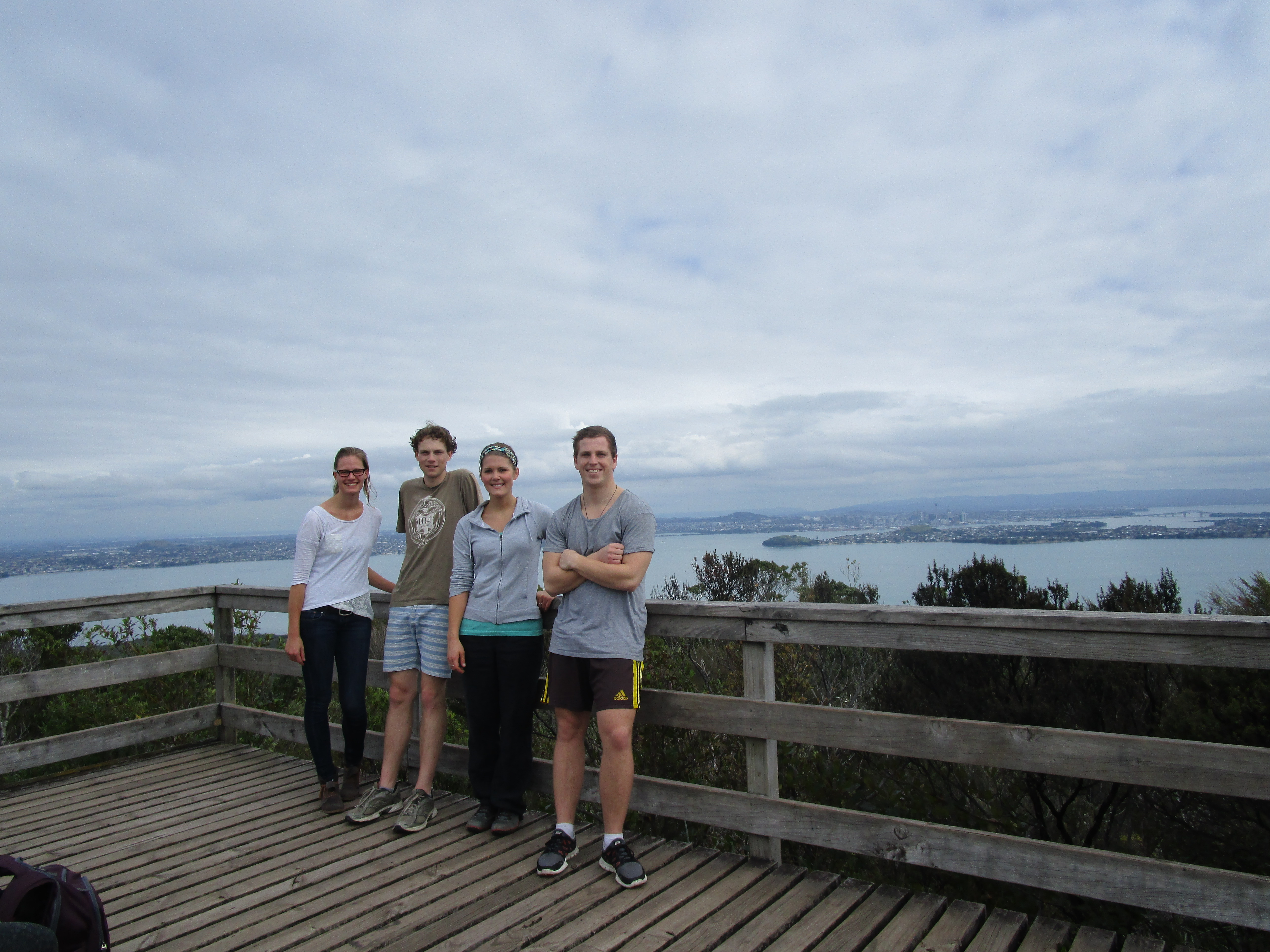 Left to right: visiting Student Miriam Timmerman from University of Twente, Sam Hitchman, Jami Johnson, and Jackson MacFarlane
As of this week, we have a sister station in Tohoku Japan: THJP. The first images coming out of this station show how seismically active that region is. Of course everyone remembers the Big Tohoku Earthquake. Our colleagues at Tohoku University have been playing an important role in understanding the underground structure, and tectonic processes that shape — and shake — Japan.

Click on this image to enlarge it. You will see the signals of several local events annotated by Dr. Kentaro Emoto using Japan’s seismic network Hi-net.
