Physical Acoustics Lab

This is an intro to  some basic tasks in seismology, performed in the python package obspy. Obspy has extensive documentation, tutorials and even a sandbox to play in, but if you are completely new to obspy, you may find the following useful.

Installations

I am going to assume you only have python on your computer, but if you have obspy and jupyter running, you can skip this section.

To get the necessary packages, I strongly encourage the use of the conda package manager. To install conda, go here.

After that, getting different python packages is a breeze. To get 2D plotting tools from matplotlib, type on the command line:

conda install matplotlib

cartopy  can be used to plot maps (there are others, such as basemap):

conda install cartopy

To get obspy, follow these simple instructions.

The following tutorials will be run in jupyter:

conda install jupyter

After this, you can run a jupyter notebook, by typing on the command line:

jupyter notebook nameofyournotebook.ipynb

These notebooks are meant to illustrate the use of obspy, in this case, but you can export the results of a jupyter notebook to html, or pdf, and even to a .py file, as a “clean” python programme.

Workflow

Let’s break down a basic seismology workflow into the tasks below. Each is a hyperlink to a notebook.

1. Building a catalogue of Earthquakes first notebook, run “jupyter notebook create_catalogue.ipynb”,
2. Creating an inventory of stations — with their instrument response — that recorded these events,
3. Retrieving seismic data from the stations in the inventory from the events in the catalogue, and performing an instrument response correction.

To avoid grainy graphics and the wrong size/type of fonts in publications and presentations, inkscape has a wonderful option, created by Johan Engelen, that splits a figure into the drawing alone and a small latex file that calls the drawing and places all fonts. When you now embed the latex file in your presentation or your publication, the latex style file will determine the size and type of the font used. The result is a perfectly embedded figure in the style of your document! Below are the steps to Nerd Nirvana:

Draw your figure

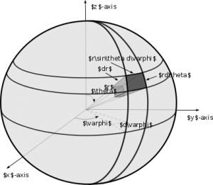
Let’s draw a figure. Here is a figure in svg-format, made in inkscape:

Note that we use latex math commands here, which makes this figure looks a bit messy, at first. When we are done drawing, we save as a pdf, and choose the option: “pdf+latex.”  The font-free pdf file is spherefigc2.pdf, and the latex file that places the fonts in it, is

%% Creator: Inkscape inkscape 0.48.5, www.inkscape.org
%% PDF/EPS/PS + LaTeX output extension by Johan Engelen, 2010
%% Accompanies image file 'spherefig2c.pdf' (pdf, eps, ps)
%%
%% To include the image in your LaTeX document, write
%%   input{<filename>.pdf_tex}
%%  instead of
%%   includegraphics{<filename>.pdf}
%% To scale the image, write
%%   defsvgwidth{<desired width>}
%%   input{<filename>.pdf_tex}
%%  instead of
%%   includegraphics[width=<desired width>]{<filename>.pdf}
%%
%% Images with a different path to the parent latex file can
%% be accessed with the `import' package (which may need to be
%% installed) using
%%   usepackage{import}
%% in the preamble, and then including the image with
%%   import{<path to file>}{<filename>.pdf_tex}
%% Alternatively, one can specify
%%   graphicspath{{<path to file>/}}
%%
%% For more information, please see info/svg-inkscape on CTAN:
%%   http://tug.ctan.org/tex-archive/info/svg-inkscape
%%
begingroup%
  makeatletter%
  providecommandcolor[2][]{%
    errmessage{(Inkscape) Color is used for the text in Inkscape, but the package 'color.sty' is not loaded}%
    renewcommandcolor[2][]{}%
  }%
  providecommandtransparent[1]{%
    errmessage{(Inkscape) Transparency is used (non-zero) for the text in Inkscape, but the package 'transparent.sty' is not loaded}%
    renewcommandtransparent[1]{}%
  }%
  providecommandrotatebox[2]{#2}%
  ifxsvgwidthundefined%
    setlength{unitlength}{565.85061095bp}%
    ifxsvgscaleundefined%
      relax%
    else%
      setlength{unitlength}{unitlength * real{svgscale}}%
    fi%
  else%
    setlength{unitlength}{svgwidth}%
  fi%
  globalletsvgwidthundefined%
  globalletsvgscaleundefined%
  makeatother%
  begin{picture}(1,0.5817873)%
    put(0,0){includegraphics[width=unitlength]{spherefig2c.pdf}}%
    put(0.34077896,0.28258916){color[rgb]{0,0,0}makebox(0,0)[lb]{smash{$r$}}}%
    put(0.58016112,0.22314528){color[rgb]{0,0,0}makebox(0,0)[lb]{smash{$y$}}}%
    put(0.02588695,0.05284654){color[rgb]{0,0,0}makebox(0,0)[lb]{smash{$x$}}}%
    put(0.26925349,0.33843429){color[rgb]{0,0,0}makebox(0,0)[lb]{smash{$theta$}}}%
    put(0.20743185,0.09461795){color[rgb]{0,0,0}makebox(0,0)[lb]{smash{$varphi$}}}%
    put(0.51123087,0.43150768){color[rgb]{0,0,0}makebox(0,0)[lb]{smash{$ {bf hat{boldsymbolvarphi}}$}}}%
    put(0.45832621,0.49970874){color[rgb]{0,0,0}makebox(0,0)[lb]{smash{${bf hat{r}}$}}}%
    put(0.47736687,0.29366584){color[rgb]{0,0,0}makebox(0,0)[lb]{smash{$ {bf hat{boldsymboltheta}}$}}}%
    put(0.18005551,0.55995116){color[rgb]{0,0,0}makebox(0,0)[lb]{smash{$z$}}}%
    put(0.25781455,0.40019168){color[rgb]{0,0,0}makebox(0,0)[lb]{smash{$(x,y,z)$}}}%
  end{picture}%
endgroup%

All that is left to do, is import this into your main latex file:

begin{figure}
    import{newfigs/}{spherefigc2.pdf_tex}
  caption{Definition of the geometric variables for an infinitesimal
    volume element $dV$ in spherical coordinates.}
  label{Sphere.figc}
end{figure}

where the end result, looks like this:

this is a low-grade snapshot of a page of our book, but if you want to see the vectorised plot, click here.

Exporting the complete figure

Some editors of journals or books may not be set up to do this dynamic handling of fonts in figures. For them, you can  “export” to a pdf file with the (correct) fonts statically embedded, you can use the package standalone.cls. Note that in the code below, we tell standalone to call the fonts from the class you want (in this case, cambridge6A.cls):

documentclass[class=cambridge6A,crop=true]{standalone}
usepackage{import}
usepackage{color}
usepackage{graphicx}
usepackage{amsmath,latexsym,amsfonts}
begin{document}
  import{newfigs/}{spherefig2c.pdf_tex}
end{document}

and its output you could call in your main latex file, in the “traditional” latex way:

begin{figure}
  includegraphics{spherefig2cwithfontsembbeded.pdf}
  caption{Definition of the geometric variables for an infinitesimal
    volume element $dV$ in spherical coordinates.}
  label{Sphere.figc}
end{figure}

As 21st century researchers, we have access to a tremendous amount of software to practice our trade. In fact, it seems every day new software appears (and some old favourites go out of style, or cease to be supported).  Below is a list of my personal favourites. The common thread here is that these are all open-source software. The reason for this is that open-source software is community supported (and often community-built). There is no messing around with the license files,  there are no black-box results (you have the source code) and even if your institution could afford the commercial programme, maybe your collaborators cannot. Or you can’t run it on your computer at home. By the way, while I shortly will advocate for the linux computer operating system, the software we list is all platform independent.

• Our operating system of choice is linux. While there is still a bit of a learning curve, installing and learning linux these days is easy. Certainly easier than it was! As is maintenance and upgrading with tools such as apt-get and dnf. There are many flavours of linux, and the differences are really not that great. Within linux, emacs is my personal favorite text editor, but there are plenty of other good ones. Gone are the days of straight-up vi!
• Our computer programs are in python, using scipy and numpy. Python is growing so fast that every time I look, there is another new part to python that makes the life of a researcher easier. Processing seismic data was done in SAC or Seismic Unix, but now there is obspy. Making maps without the commercial GIS software required Generic Mapping Tools, but now python with matplotlib, basemap and cartopy ensure vectorised figures and maps. In experiments, we control the hardware in our lab with python. Commercial options such as Labview and matlab are simply obsolete.
• Document processing is done in LaTeX. You can spot a LaTeX document from a mile away by its beautiful layout, fonts, figures, and maybe most importantly: its equations. Figure labels, section headings, equation numbers are all dynamically linked, making editing a breeze. With only a few lines difference, you can turn a paper into a presentation or a poster, too. Libreoffice, which used to be openoffice, is not bad, but often does not map one-to-one between commercial versions of Word.
• We draw in inkscape. I love all the vectorized plotting options, and LaTeX implementations with pdf outputs. Wow! Even an awful drawer like me can make something look decent.
• We tinker with arduino. Projects on school seismometers and a so-called bat-hat for a local museum rely on the wonderful open-hardware that is arduino. We foresee arduinos taking over simple lab tasks in the near future.